Welcome to the documentation of hybridLFPy!
hybridLFPy
Python module implementing a hybrid scheme for predictions of extracellular potentials (local field potentials, LFPs) of spiking neuron network simulations.
Project Status

Development
The module hybridLFPy was mainly developed in the Computational Neuroscience Group (http://compneuro.umb.no), Department of Mathemathical Sciences and Technology (http://www.nmbu.no/imt), at the Norwegian University of Life Sciences (http://www.nmbu.no), Aas, Norway, in collaboration with Institute of Neuroscience and Medicine (INM-6) and Institute for Advanced Simulation (IAS-6), Juelich Research Centre and JARA, Juelich, Germany (http://www.fz-juelich.de/inm/inm-6/EN/).
Citation
Should you find hybridLFPy useful for your research, please cite the
following paper:
Espen Hagen, David Dahmen, Maria L. Stavrinou, Henrik Lindén, Tom Tetzlaff,
Sacha J. van Albada, Sonja Grün, Markus Diesmann, Gaute T. Einevoll;
Hybrid Scheme for Modeling Local Field Potentials from Point-Neuron Networks,
Cerebral Cortex, Volume 26, Issue 12, 1 December 2016, Pages 4461–4496,
https://doi.org/10.1093/cercor/bhw237
Bibtex source:
@article{doi:10.1093/cercor/bhw237,
author = {Hagen, Espen and Dahmen, David and Stavrinou, Maria L. and Lindén,
  Henrik and Tetzlaff, Tom and van Albada, Sacha J. and Grün, Sonja and
  Diesmann, Markus and Einevoll, Gaute T.},
title = {Hybrid Scheme for Modeling Local Field Potentials from
  Point-Neuron Networks},
journal = {Cerebral Cortex},
volume = {26},
number = {12},
pages = {4461-4496},
year = {2016},
doi = {10.1093/cercor/bhw237},
URL = { + http://dx.doi.org/10.1093/cercor/bhw237},
eprint = {/oup/backfile/content_public/journal/cercor/26/12/10.1093_cercor_bhw237/2/bhw237.pdf}
}
License
- This software is released under the General Public License (see the
LICENSE file).
Warranty
This software comes without any form of warranty.
Installation
First download all the hybridLFPy source files using git
(http://git-scm.com). Open a terminal window and type:
cd $HOME/where/to/put/hybridLFPy
git clone https://github.com/INM-6/hybridLFPy.git
To use hybridLFPy from any working folder without copying files, run:
(sudo) pip install -e . (--user)
Installing it is also possible, but not recommended as things might change with future pulls from the repository:
(sudo) pip install . (--user)
examples folder
Some example script(s) on how to use this module
docs folder
Source files for autogenerated documentation using Sphinx
(https://www.sphinx-doc.org).
To compile documentation source files in this directory using sphinx, use:
sphinx-build -b html docs documentation
Dockerfile
The provided Dockerfile provides a Docker container recipe for x86_64 hosts
with all dependencies required to run simulation files provided in examples.
To build and run the container locally, get Docker from https://www.docker.com
and issue the following (replace <image-name> with a name of your choosing):
docker build -t <image-name> -< Dockerfile
docker run -it -p 5000:5000 <image-name>:latest
The --mount option can be used to mount a folder on the host to a target
folder as:
docker run --mount type=bind,source="$(pwd)",target=/opt/hybridLFPy \
-it -p 5000:5000 <image-name>
Then, code examples may be run as:
cd /opt/hybridLFPy/examples
nrnivmodl  # compile local .mod (NMODL) files
mpirun --allow-run-as-root python3 example_brunel.py
Online documentation
The sphinx-generated html documentation can be accessed at https://hybridLFPy.readthedocs.io
Notes on performance
The present version of hybridLFPy may facilitate on a trivial parallelism
as the contribution of each single-cell LFP can be computed independently.
However, this does not imply that the present implementation code is highly
optimized for speed. In particular, initializing the multicompartment neuron
populations do not as much benefit from increasing the MPI pool size, as
exemplified by a benchmark based on the Brunel-network example scaled up to
50,000 neurons and with simplified neuron morphologies.
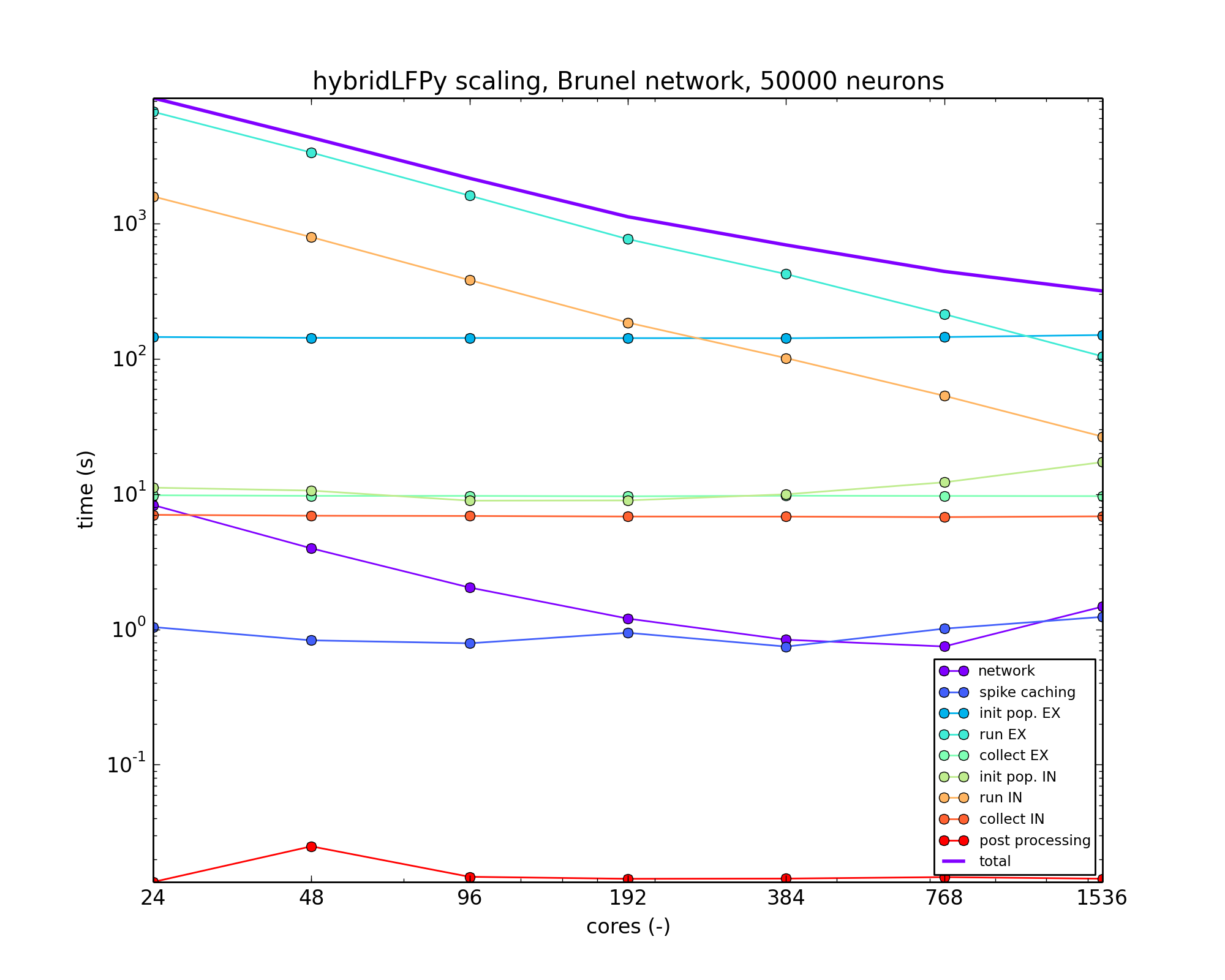
Scaling example with hybridLFPy based on a Brunel-like network with 50,000 neurons, running on the JURECA cluster at the Juelich Supercomputing Centre (JSC), Juelich Research Centre, Germany.
Module hybridLFPy
hybridLFPy
Provides methods for estimating extracellular potentials of simplified spiking neuron network models.
How to use the documentation
- Documentation is available in two forms:
Docstrings provided with the code, e.g., as hybridLFPy? within IPython
Autogenerated sphinx-built output, compiled issuing:
sphinx-build -b html docs documentation
in the root folder of the package sources
Available classes
CachedNetworkOffline interface between network spike events and used by class Population
CachedNoiseNetworkCreation of Poisson spiketrains of a putative network model, interfaces class Population
CachedFixedSpikesNetworkCreation of identical spiketrains per population of a putative network model, interface to class Population
GDFClass using sqlite to efficiently store and enquire large amounts of spike output data, used by Cached*Network
PopulationSuperParent class setting up a base population of multicompartment neurons
PopulationDaughter of PopulationSuper, using CachedNetwork spike events as synapse activation times with layer and cell type connection specificity
PostProcessMethods for processing output of multiple instances of class Population
Available utilities
helpersVarious methods used throughout simulations
setup_file_destSetup destination folders of simulation output files
testRun a series of unit tests
class CachedNetwork
- class hybridLFPy.CachedNetwork(simtime=1000.0, dt=0.1, spike_output_path='spike_output_path', label='spikes', ext='gdf', GIDs={'EX': [1, 400], 'IN': [401, 100]}, X=['EX', 'IN'], autocollect=True, skiprows=0, cmap='Dark2')[source]
Bases:
objectOffline processing and storing of network spike events, used by other class objects in the package hybridLFPy.
- Parameters
- simtimefloat
Simulation duration.
- dtfloat,
Simulation timestep size.
- spike_output_pathstr
Path to gdf/dat-files with spikes.
- labelstr
Prefix of spiking gdf/dat-files.
- extstr
File extension of gdf/dat-files.
- GIDsdict
dictionary keys are population names and value a list of length 2 with first GID in population and population size
- Xlist
names of each network population
- autocollectbool
If True, class init will process gdf/dat files.
- cmapstr
Name of colormap, must be in dir(plt.cm).
- Returns
- hybridLFPy.cachednetworks.CachedNetwork object
See also
- collect_gdf()[source]
Collect the gdf-files from network sim in folder spike_output_path into sqlite database, using the GDF-class.
- Parameters
- None
- Returns
- None
- get_xy(xlim, fraction=1.0)[source]
Get pairs of node units and spike trains on specific time interval.
- Parameters
- xlimlist of floats
Spike time interval, e.g., [0., 1000.].
- fractionfloat in [0, 1.]
If less than one, sample a fraction of nodes in random order.
- Returns
- xdict
In x key-value entries are population name and neuron spike times.
- ydict
Where in y key-value entries are population name and neuron gid number.
- plot_f_rate(ax, X, i, xlim, x, y, binsize=1, yscale='linear', plottype='fill_between', show_label=False, rasterized=False)[source]
Plot network firing rate plot in subplot object.
- Parameters
- axmatplotlib.axes.AxesSubplot object.
- Xstr
Population name.
- iint
Population index in class attribute X.
- xlimlist of floats
Spike time interval, e.g., [0., 1000.].
- xdict
Key-value entries are population name and neuron spike times.
- ydict
Key-value entries are population name and neuron gid number.
- yscale‘str’
Linear, log, or symlog y-axes in rate plot.
- plottypestr
plot type string in [‘fill_between’, ‘bar’]
- show_labelbool
whether or not to show labels
- Returns
- None
- plot_raster(ax, xlim, x, y, pop_names=False, markersize=20.0, alpha=1.0, legend=True, marker='o', rasterized=True)[source]
Plot network raster plot in subplot object.
- Parameters
- axmatplotlib.axes.AxesSubplot object
plot axes
- xlimlist
List of floats. Spike time interval, e.g., [0., 1000.].
- xdict
Key-value entries are population name and neuron spike times.
- ydict
Key-value entries are population name and neuron gid number.
- pop_names: bool
If True, show population names on yaxis instead of gid number.
- markersizefloat
raster plot marker size
- alphafloat in [0, 1]
transparency of marker
- legendbool
Switch on axes legends.
- markerstr
marker symbol for matplotlib.pyplot.plot
- rasterizedbool
if True, the scatter plot will be treated as a bitmap embedded in pdf file output
- Returns
- None
- raster_plots(xlim=[0, 1000], markersize=1, alpha=1.0, marker='o')[source]
Pretty plot of the spiking output of each population as raster and rate.
- Parameters
- xlimlist
List of floats. Spike time interval, e.g., [0., 1000.].
- markersizefloat
marker size for plot, see matplotlib.pyplot.plot
- alphafloat
transparency for markers, see matplotlib.pyplot.plot
- marker
A valid marker style
- Returns
- figmatplotlib.figure.Figure object
class CachedNoiseNetwork
- class hybridLFPy.CachedNoiseNetwork(frate={'EX': 5.0, 'IN': 10.0}, autocollect=False, **kwargs)[source]
Bases:
hybridLFPy.cachednetworks.CachedNetworkSubclass of CachedNetwork.
Use Nest to generate N_X poisson-generators each with rate frate, and record every vector, and create database with spikes.
- Parameters
- fratelist
Rate of each layer, may be tuple (onset, rate, offset)
- autocollectbool
whether or not to automatically gather gdf file output
- **kwargssee parent class hybridLFPy.cachednetworks.CachedNetwork
- Returns
- hybridLFPy.cachednetworks.CachedNoiseNetwork object
See also
class CachedFixedSpikesNetwork
- class hybridLFPy.CachedFixedSpikesNetwork(activationtimes=[200, 300, 400, 500, 600, 700, 800, 900, 1000], autocollect=False, **kwargs)[source]
Bases:
hybridLFPy.cachednetworks.CachedNetworkSubclass of CachedNetwork.
Fake nest output, where each cell in a subpopulation spike simultaneously, and each subpopulation is activated at times given in kwarg activationtimes.
- Parameters
- activationtimeslist of floats
Each entry set spike times of all cells in each population
- autocollectbool
whether or not to automatically gather gdf file output
- **kwargssee parent class hybridLFPy.cachednetworks.CachedNetwork
- Returns
- hybridLFPy.cachednetworks.CachedFixedSpikesNetwork object
See also
class PopulationSuper
- class hybridLFPy.PopulationSuper(cellParams={'Ra': 150, 'cm': 1.0, 'dt': 0.1, 'e_pas': 0.0, 'lambda_f': 100, 'morphology': 'morphologies/ex.hoc', 'nsegs_method': 'lambda_f', 'rm': 20000.0, 'tstart': 0, 'tstop': 1000.0, 'v_init': 0.0, 'verbose': False}, rand_rot_axis=[], simulationParams={}, populationParams={'min_cell_interdist': 1.0, 'number': 400, 'r_z': [[- 1e+199, 1e+99], [10, 10]], 'radius': 100, 'z_max': - 350, 'z_min': - 450}, y='EX', layerBoundaries=[[0.0, - 300], [- 300, - 500]], probes=[], savelist=['somapos'], savefolder='simulation_output_example_brunel', dt_output=1.0, recordSingleContribFrac=0, POPULATIONSEED=123456, verbose=False, output_file='{}_population_{}')[source]
Bases:
objectMain population class object, let one set up simulations, execute, and compile the results. This class is suitable for subclassing for custom cell simulation procedures, inherit things like gathering of data written to disk.
Note that PopulationSuper.cellsim do not have any stimuli, its main purpose is to gather common methods for inherited Population objects.
- Parameters
- cellParamsdict
Parameters for class LFPy.Cell
- rand_rot_axislist
Axis of which to randomly rotate morphs.
- simulationParamsdict
Additional args for LFPy.Cell.simulate().
- populationParamsdict
Constraints for population and cell number.
- ystr
Population identifier string.
- layerBoundarieslist of lists
Each element is a list setting upper and lower layer boundary (floats)
- probes: list
list of LFPykit.models.* like instances for misc. forward-model predictions
- savelistlist
LFPy.Cell arguments to save for each single-cell simulation.
- savefolderstr
path to where simulation results are stored.
- dt_outputfloat
Time resolution of output, e.g., LFP, CSD etc.
- recordSingleContribFracfloat
fraction in [0, 1] of individual neurons in population which output will be stored
- POPULATIONSEEDint/float
Random seed for population, for positions etc.
- verbosebool
Verbosity flag.
- output_filestr
formattable string for population output, e.g., ‘{}_population_{}’
- Returns
- hybridLFPy.population.PopulationSuper object
See also
Population,LFPy.Cell,LFPy.RecExtElectrode
- calc_min_cell_interdist(x, y, z)[source]
Calculate cell interdistance from input coordinates.
- Parameters
- x, y, znumpy.ndarray
xyz-coordinates of each cell-body.
- Returns
- min_cell_interdistnp.nparray
For each cell-body center, the distance to nearest neighboring cell
- calc_signal_sum(measure='LFP')[source]
Superimpose each cell’s contribution to the compound population signal, i.e., the population CSD or LFP or some other lfpykit.<instance>
- Parameters
- measurestr
- Returns
- numpy.ndarray
The populations-specific compound signal.
- cellsim(cellindex, return_just_cell=False)[source]
Single-cell LFPy.Cell simulation without any stimulus, mostly for reference, as no stimulus is added
- Parameters
- cellindexint
cell index between 0 and POPULATION_SIZE-1.
- return_just_cellbool
If True, return only the LFPy.Cell object if False, run full simulation, return None.
- Returns
- None
if `return_just_cell is False
- cellLFPy.Cell instance
if return_just_cell is True
See also
LFPy.Cell,LFPy.Synapse,LFPy.RecExtElectrode
- collectSingleContribs(measure='LFP')[source]
Collect single cell data and save them to HDF5 file. The function will also return signals generated by all cells
- Parameters
- measurestr
Either ‘LFP’, ‘CSD’ or ‘current_dipole_moment’
- Returns
- numpy.ndarray
output of all neurons in population, axis 0 correspond to neuron index
- collect_data()[source]
Collect LFPs, CSDs and soma traces from each simulated population, and save to file.
- Parameters
- None
- Returns
- None
- draw_rand_pos(radius, z_min, z_max, min_r=array([0]), min_cell_interdist=10.0, **args)[source]
Draw some random location within radius, z_min, z_max, and constrained by min_r and the minimum cell interdistance. Returned argument is a list of dicts with keys [‘x’, ‘y’, ‘z’].
- Parameters
- radiusfloat
Radius of population.
- z_minfloat
Lower z-boundary of population.
- z_maxfloat
Upper z-boundary of population.
- min_rnumpy.ndarray
Minimum distance to center axis as function of z.
- min_cell_interdistfloat
Minimum cell to cell interdistance.
- **argskeyword arguments
Additional inputs that is being ignored.
- Returns
- soma_poslist
List of dicts of len population size where dict have keys x, y, z specifying xyz-coordinates of cell at list entry i.
- run()[source]
Distribute individual cell simulations across ranks.
This method takes no keyword arguments.
- Parameters
- None
- Returns
- None
class Population
- class hybridLFPy.Population(X=['EX', 'IN'], networkSim='hybridLFPy.cachednetworks.CachedNetwork', k_yXL=[[20, 0], [20, 10]], synParams={'EX': {'section': ['apic', 'dend'], 'syntype': 'AlphaISyn'}, 'IN': {'section': ['dend'], 'syntype': 'AlphaISyn'}}, synDelayLoc=[1.5, 1.5], synDelayScale=[None, None], J_yX=[0.20680155243678455, - 1.2408093146207075], tau_yX=[0.5, 0.5], **kwargs)[source]
Bases:
hybridLFPy.population.PopulationSuperClass hybridLFPy.Population, inherited from class PopulationSuper.
This class rely on spiking times recorded in a network simulation, layer-resolved indegrees, synapse parameters, delay parameters, all per presynaptic population.
- Parameters
- Xlist of str
Each element denote name of presynaptic populations.
- networkSimhybridLFPy.cachednetworks.CachedNetwork object
Container of network spike events resolved per population
- k_yXLnumpy.ndarray
Num layers x num presynapse populations array specifying the number of incoming connections per layer and per population type.
- synParamsdict of dicts
Synapse parameters (cf. LFPy.Synapse class). Each toplevel key denote each presynaptic population, bottom-level dicts are parameters passed to LFPy.Synapse.
- synDelayLoclist
Average synapse delay for each presynapse connection.
- synDelayScalelist
Synapse delay std for each presynapse connection.
- J_yXlist of floats
Synapse weights for connections of each presynaptic population, see class LFPy.Synapse
- Returns
- hybridLFPy.population.Population object
See also
PopulationSuper,CachedNetwork,CachedFixedSpikesNetworkCachedNoiseNetwork,LFPy.Cell,LFPy.RecExtElectrode
- cellsim(cellindex, return_just_cell=False)[source]
Do the actual simulations of LFP, using synaptic spike times from network simulation.
- Parameters
- cellindexint
cell index between 0 and population size-1.
- return_just_cellbool
If True, return only the LFPy.Cell object if False, run full simulation, return None.
- Returns
- None or LFPy.Cell object
See also
hybridLFPy.csd,LFPy.Cell,LFPy.Synapse,LFPy.RecExtElectrode
- fetchSpCells(nodes, numSyn)[source]
For N (nodes count) nestSim-cells draw POPULATION_SIZE x NTIMES random cell indexes in the population in nodes and broadcast these as SpCell.
The returned argument is a list with len = numSyn.size of np.arrays, assumes numSyn is a list
- Parameters
- nodesnumpy.ndarray, dtype=int
Node # of valid presynaptic neurons.
- numSynnumpy.ndarray, dtype=int
# of synapses per connection.
- Returns
- SpCellslist
presynaptic network-neuron indices
See also
Population.fetch_all_SpCells
- fetchSynIdxCell(cell, nidx, synParams)[source]
Find possible synaptic placements for each cell As synapses are placed within layers with bounds determined by self.layerBoundaries, it will check this matrix accordingly, and use the probabilities from `self.connProbLayer to distribute.
For each layer, the synapses are placed with probability normalized by membrane area of each compartment
- Parameters
- cellLFPy.Cell instance
- nidxnumpy.ndarray
Numbers of synapses per presynaptic population X.
- synParamswhich LFPy.Synapse parameters to use.
- Returns
- syn_idxlist
List of arrays of synapse placements per connection.
See also
Population.get_all_synIdx,Population.get_synIdx,LFPy.Synapse
- get_all_SpCells()[source]
For each postsynaptic cell existing on this RANK, load or compute the presynaptic cell index for each synaptic connection
This function takes no kwargs.
- Parameters
- None
- Returns
- SpCellsdict
output[cellindex][populationname][layerindex], np.array of presynaptic cell indices.
See also
- get_all_synDelays()[source]
Create and load arrays of connection delays per connection on this rank
Get random normally distributed synaptic delays, returns dict of nested list of same shape as SpCells.
Delays are rounded to dt.
This function takes no kwargs.
- Parameters
- None
- Returns
- dict
output[cellindex][populationname][layerindex]`, np.array of delays per connection.
See also
numpy.random.normal
- get_all_synIdx()[source]
Auxilliary function to set up class attributes containing synapse locations given as LFPy.Cell compartment indices
This function takes no inputs.
- Parameters
- None
- Returns
- synIdxdict
output[cellindex][populationindex][layerindex] numpy.ndarray of compartment indices.
- get_synidx(cellindex)[source]
Local function, draw and return synapse locations corresponding to a single cell, using a random seed set as POPULATIONSEED + cellindex.
- Parameters
- cellindexint
Index of cell object.
- Returns
- synidxdict
LFPy.Cell compartment indices
- insert_all_synapses(cellindex, cell)[source]
Insert all synaptic events from all presynaptic layers on cell object with index cellindex.
- Parameters
- cellindexint
cell index in the population.
- cellLFPy.Cell instance
Postsynaptic target cell.
- Returns
- None
See also
Population.insert_synapse
- insert_synapses(cell, cellindex, synParams, idx=array([], dtype=float64), X='EX', SpCell=array([], dtype=float64), synDelays=None)[source]
Insert synapse with parameters`=`synparams on cell=cell, with segment indexes given by idx. SpCell and SpTimes picked from Brunel network simulation
- Parameters
- cellLFPy.Cell instance
Postsynaptic target cell.
- cellindexint
Index of cell in population.
- synParamsdict
Parameters passed to LFPy.Synapse.
- idxnumpy.ndarray
Postsynaptic compartment indices.
- Xstr
presynaptic population name
- SpCellnumpy.ndarray
Presynaptic spiking cells.
- synDelaysnumpy.ndarray
Per connection specific delays.
- Returns
- None
See also
class PostProcess
- class hybridLFPy.PostProcess(y=['EX', 'IN'], dt_output=1.0, mapping_Yy=[('EX', 'EX'), ('IN', 'IN')], savelist=['somapos'], probes=[], savefolder='simulation_output_example_brunel', cells_subfolder='cells', populations_subfolder='populations', figures_subfolder='figures', output_file='{}_population_{}', compound_file='{}_sum.h5')[source]
Bases:
objectclass PostProcess: Methods to deal with the contributions of every postsynaptic sub-population.
- Parameters
- ylist
Postsynaptic cell-type or population-names.
- dt_outputfloat
Time resolution of output data.
- savelistlist
List of strings, each corresponding to LFPy.Cell attributes
- probeslist
list of LFPykit.models.* like instances
- savefolderstr
Path to main output folder.
- mapping_Yylist
List of tuples, each tuple pairing population with cell type, e.g., [(‘L4E’, ‘p4’), (‘L4E’, ‘ss4’)].
- cells_subfolderstr
Folder under savefolder containing cell output.
- populations_subfolderstr
Folder under savefolder containing population specific output.
- figures_subfolderstr
Folder under savefolder containing figs.
- calc_measure(measure='LFP')[source]
Sum all the measure contributions from every cell type.
- Parameters
- measure: str
‘LFP’, ‘CSD’ or ‘current_dipole_moment’
- Returns
- measure_dict: dict of ndarray
Contributions by each cell type y
- measure_sum: ndarray
Summed contributions of all cell types
- calc_measure_layer(datadict, measure='LFP')[source]
Calculate the measure from concatenated subpopulations residing in a certain layer, e.g all L4E pops are summed, according to the mapping_Yy attribute of the hybridLFPy.Population objects.
- Parameters
- datadict: dict
- measure: str
- Returns
- measure_dict: dict of ndarray
Contributions by each subpopulation Y
class GDF
- class hybridLFPy.GDF(dbname, bsize=1000000, new_db=True, debug=False)[source]
Bases:
objectRead from gdf files.
Create sqlite db of (neuron, spike time).
Query spike times for neurons.
- Parameters
- dbnamestr
Filename of sqlite database, see sqlite3.connect
- bsizeint
Number of spike times to insert.
- new_dbbool
New database with name dbname, will overwrite at a time, determines memory usage.
- Returns
- hybridLFPy.gdf.GDF object
See also
sqlite3,sqlite3.connect,sqlite3.connect.cursor
- close()[source]
Close sqlite3.connect.cursor and sqlite3.connect objects
- Parameters
- None
- Returns
- None
See also
sqlite3.connect.cursor,sqlite3.connect
- create(re='brunel-py-ex-*.gdf', index=True, skiprows=0)[source]
Create db from list of gdf file glob
- Parameters
- restr
File glob to load.
- indexbool
Create index on neurons for speed.
- skiprowsint
Number of skipped first lines
- Returns
- None
See also
sqlite3.connect.cursor,sqlite3.connect
- create_from_list(re=[], index=True)[source]
Create db from list of arrays.
- Parameters
- relist
Index of element is cell index, and element i an array of spike times in ms.
- indexbool
Create index on neurons for speed.
- Returns
- None
See also
sqlite3.connect.cursor,sqlite3.connect
- interval(T=[0, 1000])[source]
Get all spikes in a time interval T.
- Parameters
- Tlist
Time interval.
- Returns
- slist
Nested list with spike times.
See also
sqlite3.connect.cursor
- neurons()[source]
Return list of neuron indices.
- Parameters
- None
- Returns
- list
list of neuron indices
See also
sqlite3.connect.cursor
- plotstuff(T=[0, 1000])[source]
Create a scatter plot of the contents of the database, with entries on the interval T.
- Parameters
- Tlist
Time interval.
- Returns
- None
See also
submodule helpers
Documentation:
This is a script containing general helper functions.
- hybridLFPy.helpers.autocorrfunc(freq, power)[source]
Calculate autocorrelation function(s) for given power spectrum/spectra.
- Parameters
- freqnumpy.ndarray
1 dimensional array of frequencies.
- powernumpy.ndarray
2 dimensional power spectra, 1st axis units, 2nd axis frequencies.
- Returns
- timetuple
1 dim numpy.ndarray of times.
- autoftuple
2 dim numpy.ndarray; autocorrelation functions, 1st axis units, 2nd axis times.
- hybridLFPy.helpers.calculate_fft(data, tbin)[source]
Function to calculate the Fourier transform of data.
- Parameters
- datanumpy.ndarray
1D or 2D array containing time series.
- tbinfloat
Bin size of time series (in ms).
- Returns
- freqsnumpy.ndarray
Frequency axis of signal in Fourier space.
- fftnumpy.ndarray
Signal in Fourier space.
- hybridLFPy.helpers.centralize(data, time=False, units=False)[source]
Function to subtract the mean across time and/or across units from data
- Parameters
- datanumpy.ndarray
1D or 2D array containing time series, 1st index: unit, 2nd index: time
- timebool
True: subtract mean across time.
- unitsbool
True: subtract mean across units.
- Returns
- numpy.ndarray
1D or 0D array of centralized signal.
- hybridLFPy.helpers.coherence(freq, power, cross)[source]
Calculate frequency resolved coherence for given power- and crossspectra.
- Parameters
- freqnumpy.ndarray
Frequencies, 1 dim array.
- powernumpy.ndarray
Power spectra, 1st axis units, 2nd axis frequencies.
- crossnumpy.ndarray,
Cross spectra, 1st axis units, 2nd axis units, 3rd axis frequencies.
- Returns
- freq: tuple
1 dim numpy.ndarray of frequencies.
- coh: tuple
ndim 3 numpy.ndarray of coherences, 1st axis units, 2nd axis units, 3rd axis frequencies.
- hybridLFPy.helpers.compound_crossspec(a_data, tbin, Df=None, pointProcess=False)[source]
Calculate cross spectra of compound signals. a_data is a list of datasets (a_data = [data1,data2,…]). For each dataset in a_data, the compound signal is calculated and the crossspectra between these compound signals is computed.
If pointProcess=True, power spectra are normalized by the length T of the time series.
- Parameters
- a_datalist of numpy.ndarrays
Array: 1st axis unit, 2nd axis time.
- tbinfloat
Binsize in ms.
- Dffloat/None,
Window width of sliding rectangular filter (smoothing), None -> no smoothing.
- pointProcessbool
If set to True, crossspectrum is normalized to signal length T
- Returns
- freqtuple
numpy.ndarray of frequencies.
- CROtuple
3 dim numpy.ndarray; 1st axis first compound signal, 2nd axis second compound signal, 3rd axis frequency.
Examples
>>> compound_crossspec([np.array([analog_sig1, analog_sig2]),
                        np.array([analog_sig3,analog_sig4])], tbin, Df=Df)
Out[1]: (freq,CRO)
>>> CRO.shape
Out[2]: (2,2,len(analog_sig1))
- hybridLFPy.helpers.compound_mean(data)[source]
Compute the mean of the compound/sum signal. Data is first summed across units and averaged across time.
- Parameters
- datanumpy.ndarray
1st axis unit, 2nd axis time
- Returns
- float
time-averaged compound/sum signal
Examples
>>> compound_mean(np.array([[1, 2, 3], [4, 5, 6]]))
7.0
- hybridLFPy.helpers.compound_powerspec(data, tbin, Df=None, pointProcess=False)[source]
Calculate the power spectrum of the compound/sum signal. data is first summed across units, then the power spectrum is calculated.
If pointProcess=True, power spectra are normalized by the length T of the time series.
- Parameters
- datanumpy.ndarray,
1st axis unit, 2nd axis time
- tbinfloat,
binsize in ms
- Dffloat/None,
window width of sliding rectangular filter (smoothing), None -> no smoothing
- pointProcessbool,
if set to True, powerspectrum is normalized to signal length T
- Returns
- freqtuple
numpy.ndarray of frequencies
- POWtuple
1 dim numpy.ndarray, frequency series
Examples
>>> compound_powerspec(np.array([analog_sig1, analog_sig2]), tbin, Df=Df)
Out[1]: (freq,POW)
>>> POW.shape
Out[2]: (len(analog_sig1),)
- hybridLFPy.helpers.compound_variance(data)[source]
Compute the variance of the compound/sum signal. Data is first summed across units, then the variance across time is calculated.
- Parameters
- datanumpy.ndarray
1st axis unit, 2nd axis time
- Returns
- float
variance across time of compound/sum signal
Examples
>>> compound_variance(np.array([[1, 2, 3], [4, 5, 6]]))
2.6666666666666665
- hybridLFPy.helpers.corrcoef(time, crossf, integration_window=0.0)[source]
Calculate the correlation coefficient for given auto- and crosscorrelation functions. Standard settings yield the zero lag correlation coefficient. Setting integration_window > 0 yields the correlation coefficient of integrated auto- and crosscorrelation functions. The correlation coefficient between a zero signal with any other signal is defined as 0.
- Parameters
- timenumpy.ndarray
1 dim array of times corresponding to signal.
- crossfnumpy.ndarray
Crosscorrelation functions, 1st axis first unit, 2nd axis second unit, 3rd axis times.
- integration_window: float
Size of the integration window.
- Returns
- ccnumpy.ndarray
2 dim array of correlation coefficient between two units.
- hybridLFPy.helpers.crosscorrfunc(freq, cross)[source]
Calculate crosscorrelation function(s) for given cross spectra.
- Parameters
- freqnumpy.ndarray
1 dimensional array of frequencies.
- crossnumpy.ndarray
2 dimensional array of cross spectra, 1st axis units, 2nd axis units, 3rd axis frequencies.
- Returns
- timetuple
1 dim numpy.ndarray of times.
- crossftuple
3 dim numpy.ndarray, crosscorrelation functions, 1st axis first unit, 2nd axis second unit, 3rd axis times.
- hybridLFPy.helpers.crossspec(data, tbin, Df=None, units=False, pointProcess=False)[source]
Calculate (smoothed) cross spectra of data. If `units`=True, cross spectra are averaged across units. Note that averaging is done on cross spectra rather than data.
Cross spectra are normalized by the length T of the time series -> no scaling with T.
If pointProcess=True, power spectra are normalized by the length T of the time series.
- Parameters
- datanumpy.ndarray,
1st axis unit, 2nd axis time
- tbinfloat,
binsize in ms
- Dffloat/None,
window width of sliding rectangular filter (smoothing), None -> no smoothing
- unitsbool,
average cross spectrum
- pointProcessbool,
if set to True, cross spectrum is normalized to signal length T
- Returns
Examples
>>> crossspec(np.array([analog_sig1, analog_sig2]), tbin, Df=Df)
Out[1]: (freq,CRO)
>>> CRO.shape
Out[2]: (2,2,len(analog_sig1))
>>> crossspec(np.array([analog_sig1, analog_sig2]), tbin, Df=Df, units=True)
Out[1]: (freq,CRO)
>>> CRO.shape
Out[2]: (len(analog_sig1),)
- hybridLFPy.helpers.cv(data, units=False)[source]
Calculate coefficient of variation (cv) of data. Mean and standard deviation are computed across time.
- Parameters
- datanumpy.ndarray
1st axis unit, 2nd axis time.
- unitsbool
Average cv.
- Returns
- numpy.ndarray
If units=False, series of unit `cv`s.
- float
If units=True, mean cv across units.
Examples
>>> cv(np.array([[1, 2, 3, 4, 5, 6], [11, 2, 3, 3, 4, 5]]))
array([ 0.48795004,  0.63887656])
>>> cv(np.array([[1, 2, 3, 4, 5, 6], [11, 2, 3, 3, 4, 5]]), units=True)
0.56341330073710316
- hybridLFPy.helpers.dump_dict_of_nested_lists_to_h5(fname, data)[source]
Take nested list structure and dump it in hdf5 file.
- Parameters
- fnamestr
Filename
- datadict(list(numpy.ndarray))
Dict of nested lists with variable len arrays.
- Returns
- None
- hybridLFPy.helpers.fano(data, units=False)[source]
Calculate fano factor (FF) of data. Mean and variance are computed across time.
- Parameters
- datanumpy.ndarray
1st axis unit, 2nd axis time.
- unitsbool
Average FF.
- Returns
- numpy.ndarray
If units=False, series of unit FFs.
- float
If units=True, mean FF across units.
Examples
>>> fano(np.array([[1, 2, 3, 4, 5, 6], [11, 2, 3, 3, 4, 5]]))
array([ 0.83333333,  1.9047619 ])
>>> fano(np.array([[1, 2, 3, 4, 5, 6], [11, 2, 3, 3, 4, 5]]), units=True)
1.3690476190476191
- hybridLFPy.helpers.load_dict_of_nested_lists_from_h5(fname, toplevelkeys=None)[source]
Load nested list structure from hdf5 file
- Parameters
- fnamestr
Filename
- toplevelkeysNone or iterable,
Load a two(default) or three-layered structure.
- Returns
- dict(list(numpy.ndarray))
dictionary of nested lists with variable length array data.
- hybridLFPy.helpers.load_h5_data(path='', data_type='LFP', y=None, electrode=None, warmup=0.0, scaling=1.0)[source]
Function loading results from hdf5 file
- Parameters
- pathstr
Path to hdf5-file
- data_typestr
Signal types in [‘CSD’ , ‘LFP’, ‘CSDsum’, ‘LFPsum’].
- yNone or str
Name of population.
- electrodeNone or int
TODO: update, electrode is NOT USED
- warmupfloat
Lower cutoff of time series to remove possible transients
- scalingfloat,
Scaling factor for population size that determines the amount of loaded single-cell signals
- Returns
- numpy.ndarray
[electrode id, compound signal] if y is None
- numpy.ndarray
[cell id, electrode, single-cell signal] otherwise
- hybridLFPy.helpers.mean(data, units=False, time=False)[source]
Function to compute mean of data
- Parameters
- datanumpy.ndarray
1st axis unit, 2nd axis time
- unitsbool
Average over units
- timebool
Average over time
- Returns
- if units=False and time=False:
error
- if units=True:
1 dim numpy.ndarray; time series
- if time=True:
1 dim numpy.ndarray; series of unit means across time
- if units=True and time=True:
float; unit and time mean
Examples
>>> mean(np.array([[1, 2, 3], [4, 5, 6]]), units=True)
array([ 2.5,  3.5,  4.5])
>>> mean(np.array([[1, 2, 3], [4, 5, 6]]), time=True)
array([ 2.,  5.])
>>> mean(np.array([[1, 2, 3], [4, 5, 6]]), units=True,time=True)
3.5
- hybridLFPy.helpers.movav(y, Dx, dx)[source]
Moving average rectangular window filter: calculate average of signal y by using sliding rectangular window of size Dx using binsize dx
- Parameters
- ynumpy.ndarray
Signal
- Dxfloat
Window length of filter.
- dxfloat
Bin size of signal sampling.
- Returns
- numpy.ndarray
Filtered signal.
- hybridLFPy.helpers.normalize(data)[source]
Function to normalize data to have mean 0 and unity standard deviation (also called z-transform)
- Parameters
- datanumpy.ndarray
- Returns
- numpy.ndarray
z-transform of input array
- hybridLFPy.helpers.powerspec(data, tbin, Df=None, units=False, pointProcess=False)[source]
Calculate (smoothed) power spectra of all timeseries in data. If units=True, power spectra are averaged across units. Note that averaging is done on power spectra rather than data.
If pointProcess is True, power spectra are normalized by the length T of the time series.
- Parameters
- datanumpy.ndarray
1st axis unit, 2nd axis time.
- tbinfloat
Binsize in ms.
- Dffloat/None,
Window width of sliding rectangular filter (smoothing), None is no smoothing.
- unitsbool
Average power spectrum.
- pointProcessbool
If set to True, powerspectrum is normalized to signal length T.
- Returns
- freqtuple
numpy.ndarray of frequencies.
- POWtuple
- if units=False:
2 dim numpy.ndarray; 1st axis unit, 2nd axis frequency
- if units=True:
1 dim numpy.ndarray; frequency series
Examples
>>> powerspec(np.array([analog_sig1, analog_sig2]), tbin, Df=Df)
Out[1]: (freq,POW)
>>> POW.shape
Out[2]: (2,len(analog_sig1))
>>> powerspec(np.array([analog_sig1, analog_sig2]), tbin, Df=Df, units=True)
Out[1]: (freq,POW)
>>> POW.shape
Out[2]: (len(analog_sig1),)
- hybridLFPy.helpers.read_gdf(fname, skiprows=0)[source]
Fast line-by-line gdf-file reader.
- Parameters
- fnamestr
Path to gdf-file.
- skiprowsint
number of skipped rows
- Returns
- numpy.ndarray
([gid, val0, val1, **]), dtype=object) mixed datatype array
- hybridLFPy.helpers.setup_file_dest(params, clearDestination=True)[source]
Function to set up the file catalog structure for simulation output
- Parameters
- paramsobject
e.g., cellsim16popsParams.multicompartment_params()
- clear_destbool
Savefolder will be cleared if already existing.
- Returns
- None
- hybridLFPy.helpers.variance(data, units=False, time=False)[source]
Compute the variance of data across time, units or both.
- Parameters
- datanumpy.ndarray
1st axis unit, 2nd axis time.
- unitsbool
Variance across units
- timebool
Average over time
- Returns
- if units=False and time=False:
Exception
- if units=True:
1 dim numpy.ndarray; time series
- if time=True:
1 dim numpy.ndarray; series of single unit variances across time
- if units=True and time=True:
float; mean of single unit variances across time
Examples
>>> variance(np.array([[1, 2, 3],[4, 5, 6]]), units=True)
array([ 2.25,  2.25,  2.25])
>>> variance(np.array([[1, 2, 3], [4, 5, 6]]), time=True)
array([ 0.66666667,  0.66666667])
>>> variance(np.array([[1, 2, 3], [4, 5, 6]]), units=True, time=True)
0.66666666666666663
submodulue test
- hybridLFPy.test(verbosity=2)
Run unittests for hybridLFPy
- Returns
- None